PiggyCast: Improving weather prediction skill through a stacking-based ensemble AI approach.
We argue that the future of the most skilful weather forecasts will likely come from machine learning stacking, by the very nature that stacking typically yields performance beyond than any base model
In this post, Josiah summarises his MSc thesis, highlighting the key results. He was supervised by Oliver Angélil & Chris Toumping.
Introduction
Accurate weather prediction is crucial in disaster preparedness, resource management, and societal resilience. Traditionally, Numerical Weather Prediction (NWP) models, which rely on dynamical and physics-based simulations of atmospheric processes, have been the cornerstone of weather forecasting. Despite their proven skill, these models face computational challenges and sensitivity to initial conditions, especially when producing high-resolution and long-range forecasts.
Recent advances in Artificial Intelligence Weather Prediction (AIWP) leverage machine learning techniques to complement or even replace traditional NWP models. AIWP models efficiently learn complex patterns from large datasets, correct systematic biases in dynamical models, and offer substantial gains in computational efficiency. However, purely data-driven approaches often lack physical interpretability and may struggle to generalise to unseen climate conditions or extreme weather events.
Hybrid forecasting systems have emerged to combine the strengths of both paradigms, integrating physics-based and data-driven predictions to improve forecast skill across various meteorological variables, including rainfall, temperature, and extreme weather phenomena.
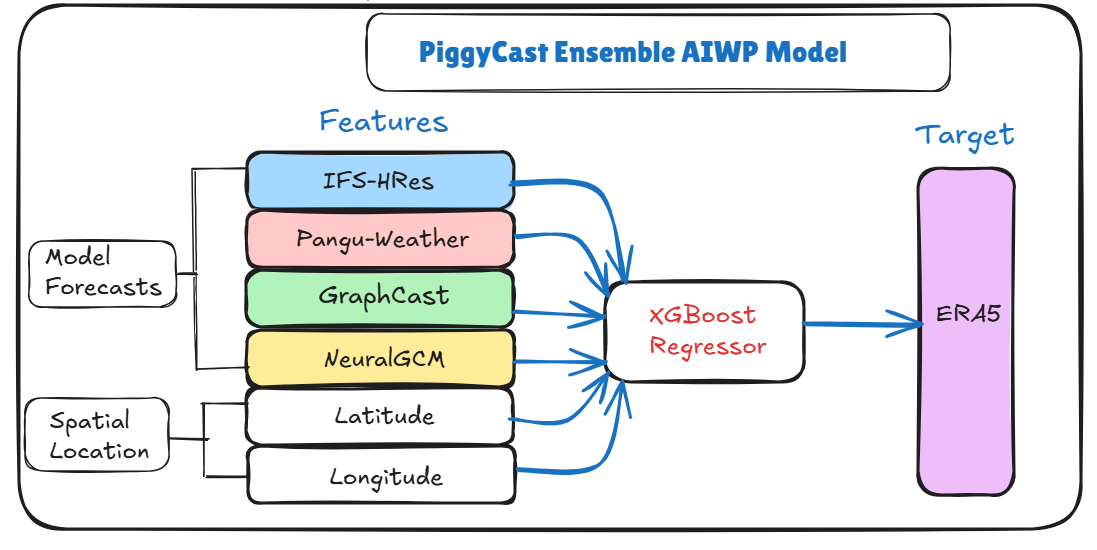
Building on these developments, this study proposes an ensemble machine learning model trained on the forecasts from these models using a stacking approach, demonstrating that such a combined model can outperform any individual base model. We coined our model “PiggyCast”, as we effectively piggyback off the work done by leading AI research teams with expertise and compute budgets for model training that are hard to match in an MSc thesis.
Additionally, we investigate the interpretability of the ensemble’s input features to improve understanding of the forecasting process.
Data Source and Models
Concurrently, benchmarking initiatives like WeatherBench have standardised the evaluation of NWP, AI, and hybrid models, facilitating direct comparisons across datasets and metrics.
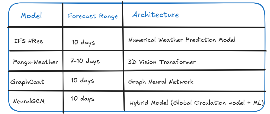
The ERA5 global atmospheric reanalysis dataset serves as the ground truth. Forecasts from four state-of-the-art weather prediction models—IFS HRES, GraphCast, Pangu Weather, and NeuralGCM—are evaluated against the ERA5 data. All data were accessed via the WeatherBench 2 (WB2) framework.
The study focuses on a single key meteorological variable: geopotential height at the 500 hPa pressure level, evaluated globally over 9 lead times (from 48 to 240 hours in 24-hour intervals). The choice of this variable is guided by its long-standing importance in meteorological research and performance evaluation in forecasting.
Data are downsampled to a 5.625-degree (64 longitude * 32 latitude) resolution and temporally subsampled to 12-hour intervals for computational tractability. The year 2020 was selected for analysis.
Methodology: PiggyCast Ensemble
XGBoost Regressor
XGBoost (Extreme Gradient Boosting) is a scalable and efficient implementation of gradient boosting machines, introduced by Chen in 2016 (xgboost paper). The model constructs an ensemble of regression trees in an additive manner, where each new tree is trained to correct the residual errors of the previous trees.
A key innovation of XGBoost lies in its regularised objective function and the use of second-order Taylor expansion, which contribute significantly to both its predictive performance and computational efficiency.
Learning Objective Function
The learning objective in XGBoost consists of a differentiable loss function that measures the model's fit and a regularisation term that penalises model complexity:
Let
denote the forecasted value at spatial location x and lead time
hours by model i.
The feature vector for each instance is defined as:
with the target variable:
The loss function around
where
is the first-order gradient, and
is the second-order derivative (Hessian).
Evaluation Metrics
1. Area-weighted RMSE
Let M1 and M2 represent the ERA5 value and a model spatial forecast, respectively, then
where
is the area weight for grid point i on latitude Φ, and n is the number of grid points.
2. Model Performance Across Lead Times
For each fold (time series cross-validation split) and model, we compute the RMSE & average across folds:
where m is the model and K=10 is the number of folds.
Feature Attribution: SHAP (SHapley Additive exPlanations) Values
Given the trained model f and input x, the SHAP value Φ_j for feature j represents the marginal contribution of that feature:
where Φ_0 is the base value (mean model output) and M is the number of input features
Results and Discussion
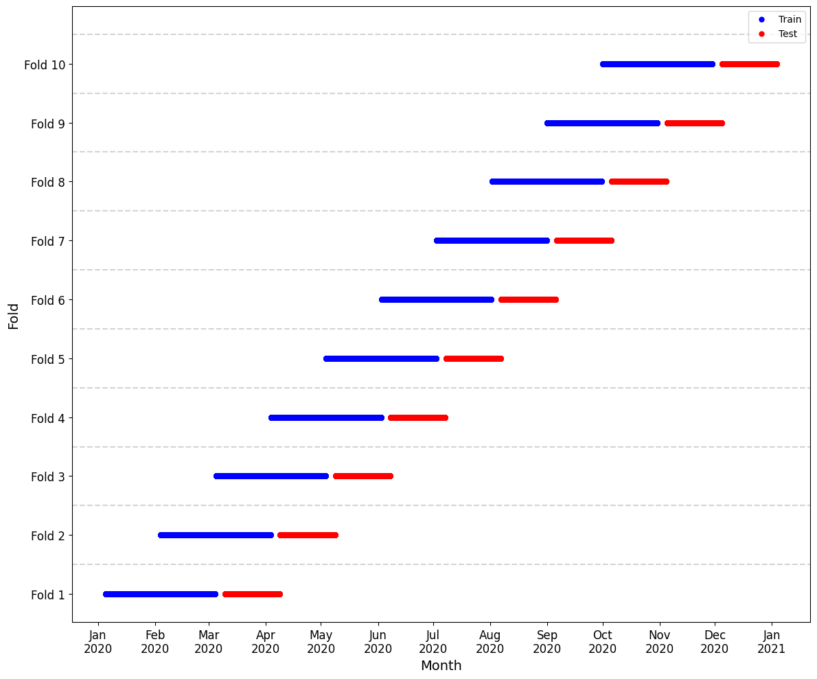
In our implementation, we use a 10-fold time series cross-validation split, with each fold comprising:
Training set: 64 * 32 * 2 * 60 time steps (60 days of training)
Gap: 64 * 32 * 2 * 5 time steps (5 days as autocorrelation gap)
Test set: 64 * 32 * 2 * 30 time steps (30 days of testing)
where 64 * 32 * 2 are the longitude and latitude geopotential height values evaluated twice in a day (noon and midnight), as shown in the figure below
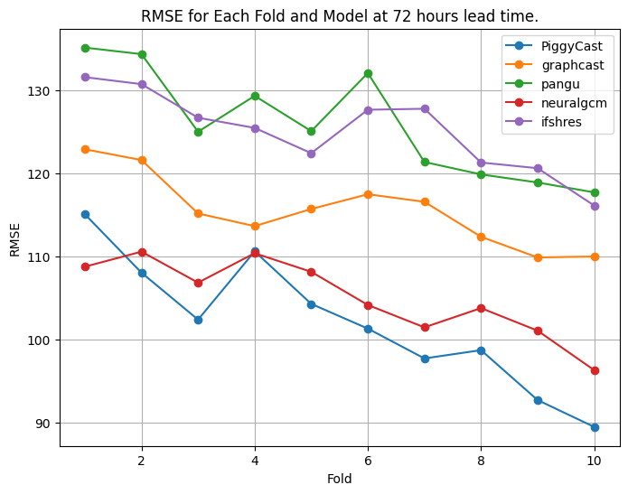
At a 72-hour lead time, PiggyCast performance is noted to improve and provides the best predictions compared to the other models, as shown below.
It is only at fold one where NeuralGCM outperforms PiggyCast, while at fold four, NeuralGCM matches the performance of PiggyCast. On average (across folds), PiggyCast's RMSE leads with 101.99 m, followed by NeuralGCM (105.11 m), GraphCast (115.48 m), IFS HRES (124.99 m) and finally Pangu (125.84 m).
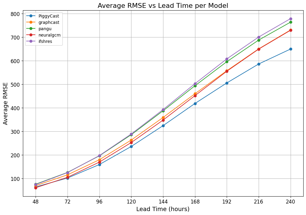
To evaluate the models' performance across 48-240 hour lead times, we calculate and plot the average RMSE across folds for each model per time lead as shown below.
PiggyCast's dominance is observed as the lead time increases. NeuralGCM starts strong but converges with GraphCast from 192-240 hours lead times. Similarly, IFS HRES and Pangu performance are similar but diverge from 140-240 hours lead times.
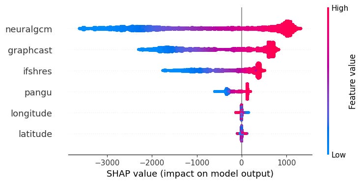
We attempt to gain insight into PiggyCast's decision-making process and explain the contribution of features of the model by using SHAPley (SHAP) values. The Figure below visualises the local contribution of each feature by either decreasing (negative SHAP values in blue) or increasing (positive SHAP values in red) the base value of each prediction for a 72-hour lead time.
From the bee-swarm plot, we observe that NeuralGCM, GraphCast and IFS HRES greatly influence PiggyCast's decision-making at each prediction as seen with long and densely populated tails on either side of the zero divide. Pangu, longitude and latitude contribute the least to the prediction of the model, as seen with the short tails that are centred at zero.
Conclusion
Given the low compute cost of making forecasts, and that each frontier AIWP model has its strengths and limitations (depending on the weather variable, region of the globe, and forecast lead time), we argue that the future of the most skilful weather forecasts will likely come from machine learning stacking, by the very nature that stacking typically yields performance better than any base model alone.
Nonetheless, several avenues remain open for future exploration. These include:
Incorporation of additional weather variables and weather forecasting models.
Testing the sensitivity of PiggyCast, relative to the best base model, to the spatial scale of a region. Since in this study we optimise for weather globally, we suspect that when targeting smaller spatial scales, PiggyCast may exhibit impressive results.
Extension of the framework to address extreme weather events, non-stationary climate conditions and uncertainty quantification.
Code Availability
The code and detailed exploration of this research are made publicly available on the GitHub repo here.




Almost like WeatherUnderground meets AI. Loved the SHAP value chart.
This is really interesting work! Did you experiment with any other methods besides the XGBoost Regressor to "stack" the model outputs?